\\\\( \nonumber \newcommand{\bevisslut}{$\blacksquare$} \newenvironment{matr}[1]{\hspace{-.8mm}\begin{bmatrix}\hspace{-1mm}\begin{array}{#1}}{\end{array}\hspace{-1mm}\end{bmatrix}\hspace{-.8mm}} \newcommand{\transp}{\hspace{-.6mm}^{\top}} \newcommand{\maengde}[2]{\left\lbrace \hspace{-1mm} \begin{array}{c|c} #1 & #2 \end{array} \hspace{-1mm} \right\rbrace} \newenvironment{eqnalign}[1]{\begin{equation}\begin{array}{#1}}{\end{array}\end{equation}} \newcommand{\eqnl}{} \newcommand{\matind}[3]{{_\mathrm{#1}\mathbf{#2}_\mathrm{#3}}} \newcommand{\vekind}[2]{{_\mathrm{#1}\mathbf{#2}}} \newcommand{\jac}[2]{{\mathrm{Jacobi}_\mathbf{#1} (#2)}} \newcommand{\diver}[2]{{\mathrm{div}\mathbf{#1} (#2)}} \newcommand{\rot}[1]{{\mathbf{rot}\mathbf{(#1)}}} \newcommand{\am}{\mathrm{am}} \newcommand{\gm}{\mathrm{gm}} \newcommand{\E}{\mathrm{E}} \newcommand{\Span}{\mathrm{span}} \newcommand{\mU}{\mathbf{U}} \newcommand{\mA}{\mathbf{A}} \newcommand{\mB}{\mathbf{B}} \newcommand{\mC}{\mathbf{C}} \newcommand{\mD}{\mathbf{D}} \newcommand{\mE}{\mathbf{E}} \newcommand{\mF}{\mathbf{F}} \newcommand{\mK}{\mathbf{K}} \newcommand{\mI}{\mathbf{I}} \newcommand{\mM}{\mathbf{M}} \newcommand{\mN}{\mathbf{N}} \newcommand{\mQ}{\mathbf{Q}} \newcommand{\mT}{\mathbf{T}} \newcommand{\mV}{\mathbf{V}} \newcommand{\mW}{\mathbf{W}} \newcommand{\mX}{\mathbf{X}} \newcommand{\ma}{\mathbf{a}} \newcommand{\mb}{\mathbf{b}} \newcommand{\mc}{\mathbf{c}} \newcommand{\md}{\mathbf{d}} \newcommand{\me}{\mathbf{e}} \newcommand{\mn}{\mathbf{n}} \newcommand{\mr}{\mathbf{r}} \newcommand{\mv}{\mathbf{v}} \newcommand{\mw}{\mathbf{w}} \newcommand{\mx}{\mathbf{x}} \newcommand{\mxb}{\mathbf{x_{bet}}} \newcommand{\my}{\mathbf{y}} \newcommand{\mz}{\mathbf{z}} \newcommand{\reel}{\mathbb{R}} \newcommand{\mL}{\bm{\Lambda}} \newcommand{\mnul}{\mathbf{0}} \newcommand{\trap}[1]{\mathrm{trap}(#1)} \newcommand{\Det}{\operatorname{Det}} \newcommand{\adj}{\operatorname{adj}} \newcommand{\Ar}{\operatorname{Areal}} \newcommand{\Vol}{\operatorname{Vol}} \newcommand{\Rum}{\operatorname{Rum}} \newcommand{\diag}{\operatorname{\bf{diag}}} \newcommand{\bidiag}{\operatorname{\bf{bidiag}}} \newcommand{\spanVec}[1]{\mathrm{span}{#1}} \newcommand{\Div}{\operatorname{Div}} \newcommand{\Rot}{\operatorname{\mathbf{Rot}}} \newcommand{\Jac}{\operatorname{Jacobi}} \newcommand{\Tan}{\operatorname{Tan}} \newcommand{\Ort}{\operatorname{Ort}} \newcommand{\Flux}{\operatorname{Flux}} \newcommand{\Cmass}{\operatorname{Cm}} \newcommand{\Imom}{\operatorname{Im}} \newcommand{\Pmom}{\operatorname{Pm}} \newcommand{\IS}{\operatorname{I}} \newcommand{\IIS}{\operatorname{II}} \newcommand{\IIIS}{\operatorname{III}} \newcommand{\Le}{\operatorname{L}} \newcommand{\app}{\operatorname{app}} \newcommand{\M}{\operatorname{M}} \newcommand{\re}{\mathrm{Re}} \newcommand{\im}{\mathrm{Im}} \newcommand{\compl}{\mathbb{C}} \newcommand{\e}{\mathrm{e}} \\\\)

Time Series Analysis
- with a focus on modelling and forecasting in energy systems Summer School

Venue: TBA (somewhere in Denmark, last year Maskinmesterskolen Fredericia ) Date: August 19-23, 2024.

To integrate renewable and fluctuating power generation sources we need to model, forecast and optimize the operation of distributed energy resources, hence we need self tuning models for each component in the system. E.g. for a building with PV and a heat pump, one will need a model from weather forecasts and control variables to PV power, heat pump load and the indoor temperature in the building. These, together with electricity prices, can then be used for MPC of the heat pump to shift its load to match the generation of power. There are many other applications of data-driven models, eg. performance assessment, flexibility characterization, and fault-detection; these topics will also be presented. The statistical techniques behind the models will be elaborated, with focus on non-parametric (e.g. kernels and splines) models, discrete and continuous time models (grey-box modelling with SDEs).

We will use R and provide exercises to get a “hands-on” experience with the techniques. The summer school will be held for the seventh time by DTU. PhD students completing the course will achieve 2.5 ECTS points. There will be a fee of 300 Euros for participating (higher for industry participants). A social event and dinner is included. We offer no online participation.

A student who has met the learning objectives of the course will be able to:

  • Achieve a thorough understanding of maximum likelihood estimation techniques.
  • Formulate and apply non-parametric models using kernel functions and splines - with a focus on solar and occupancy effects.
  • Formulate and apply time adaptive models.
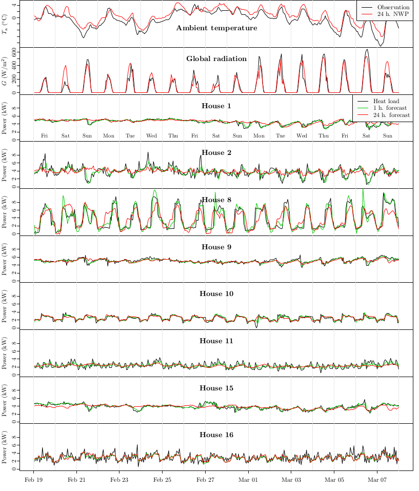
  • Formulate and apply models for short-term forecasting in energy systems, e.g. for heat load in buildings, electrical power from PV and wind systems. Application of statistical model selection techniques (AIC, BIC, likelihood-ratio tests, model validation).
  • Formulate and apply grey-box and digital twin models - model identification - tests for model order and model validation, and advanced non-linear models.
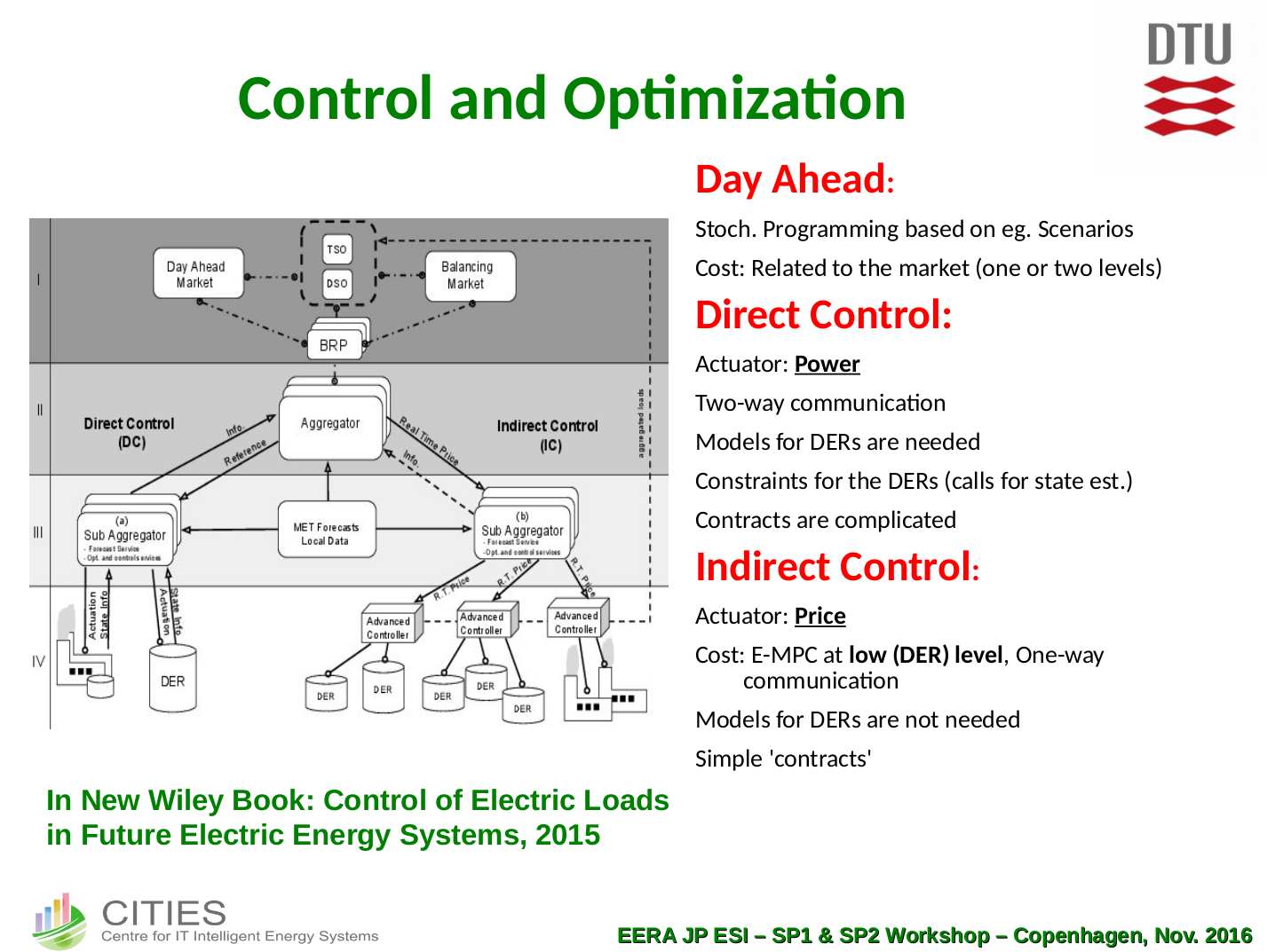
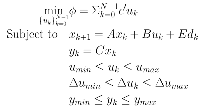
  • Achieve an understanding of model predictive control (MPC) via applied examples on energy systems.
  • Achieve an understanding of flexibility functions and indices.

The summer school is held by DTU in a collaboration with Center Denmark, Maskinmesterskolen and IEA EBC Annexes 81, 82 and 83, and the projects Next Energy, DEH, ARV, syn.ikia, BIPED, Seeds, Begonia and Elexia. For more information, contact Henrik Madsen (mailto:hmad@dtu.dk) or Peder Bacher (mailto:pbac@dtu.dk). See also this description of DTU course 02960.

Logoes